Economic order quantity

Definition; specific objectives; definition; eoq assumptions; eoq cost breakdown; eoq mathematical & graphical models; advantages

Specific objectives

This article is guided by the following 11 specific objectives. The learner/user of this article will be able to;

1. 1. Define the term Economic Order Quantity (EOQ)
   2. Describe the assumptions of EOQ Model
   3. Empirically derive at the EOQ model
   4. Analyze EOQ cost breakdown
   5. Demonstrate the relationship between ordering cost and holding cost
   6. Derive at the graphical EOQ model using available information
   7. Explain the advantages and disadvantages of EOQ model

Definition

Economic Order Quantity (EOQ) is a stock management tool or model that is used to determine the most appropriate or ideal stock size or re-order quantity for the business. It is a model that guides the management on the size of an order (units) placed.

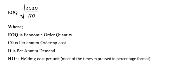
The EOQ model represents the quantity to be purchased per order with the lowest total cost per order. On one extreme side, it entails the Holding costs (H) and on the other side Ordering costs. The model is commonly presented in mathematical and graph format as expressed below.

Assumptions of economic order quantity (eoq)

1. EOQ associated holding cost is fixed.
2. There is certainty in demand level.
3. Delivery of placed orders is perfect.
4. No disruptions in delivery.
5. There exist fixed inventory costs under EOQ approach.

For EOQ model to function, the following assumptions has to be adopted

EOQ Cost Breakdown

As stated earlier, the EOQ model is made up of two mainstream costs. On one end the ordering cost and on the other the holding cost. The analysis which follows is for your in-depth understanding and appreciation of the model in its applicability.

Ordering Cost

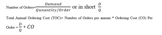
Ordering Cost (CO) is the expenses or economic resources used to order inventory in a year (i.e., per annum). The inventory is acquired in terms of orders placed for supply by the sellers. The total orders made in a year are determined by the demand level in a year commonly referred to as Normal Consumption (NC) or usage. Note that the higher the demand level, the more the number of orders and the vice versa is true.

Ordering cost is in terms of Fixed Cost (FC) per order and therefore, the more the number of orders per annum the more the Total Ordering Cost (TOC) and the less the number of orders the less the TOC.

Therefore, if the total demand of raw materials or finished goods is known, to determine the total number of orders is established by dividing the total demand level with the size of one order made for it is assumed to contain uniform units of goods. So, the number of orders will be;

Holding Cost

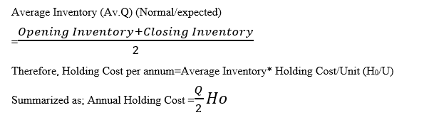
Holding cost is the economic resources (i.e., expenses incurred or paid) used in holding the inventory once it is delivered in the premises of the business by the supplier(s). The costs of holding inventory can be direct or indirect. For example, the interest paid for accessing a financing facility to hold the stock such as interest on loan. Or it can be an indirect cost such as opportunity cost, we have mentioned earlier on. In this case of holding inventory, the opportunity cost relevant here can be something such as benefits that could have been derived from investing the inventory money in another profitable venture. The Total Holding Cost (THC) is measured in terms of holding cost multiplied by inventory in a year (i.e., per annum).

But you see, inventory in a year is two, the opening inventory and the closing inventory. Therefore, to determine average inventory/expected inventory we determine the average inventory as follows;

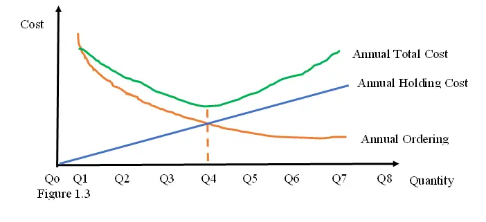
Relationship between Ordering Cost and Holding Cost

When the number of orders increase, the ordering cost decreases due to the advantages derived from the economies of scale rule. Such that, as more orders are being placed, the less the ordering cost. On the other hand, as more orders are being made, it means that the holding cost for inventory thereof increases. Therefore, the relationship between the ordering cost and holding cost is inverse. Such that as the ordering cost increase, the holding cost decrease and when ordering cost decrease, the holding costs increase.

This relationship between ordering cost and holding cost prompts the purchasing manager to strike a balance between the two extreme cost to appoint where total cost (summation of the two types of cost) is at the lowest ebb. At this point now, let us look at how to derive at the EOQ formula or model by incorporating the two costs (total cost) for a year (annum) and the Economic order quantity.

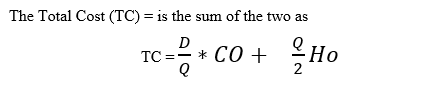
At this point, we will further borrow a leaf from Economics discipline on matters of a profit maximizing firm and choice of resources. It is argued that for a profit maximizing firm, it will achieve the objective of optimizing this choice of resources such as inventory level by carrying out first and second partial differentiation. In the first step of differentiation, the condition is that the total cost function or model should be equal to zero. Let me not go to the second condition for this is not our main focus but you can refer to any Micro-Economics text book. So, if we re-visit our total cost model above, and then differentiate it, this are the results;

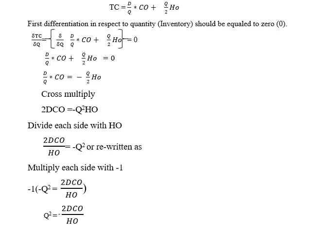
Compute the square root. Then the mathematical EOQ Model becomes….

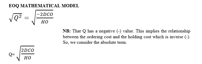
Where;

Q is the Economic Order Quantity (EOQ).

D is the demand per annum (i.e., Average stock).

CO is the per annum ordering cost.

HO is the per annum holding cost.

NB: These types of costs may not be directly stated in the question and as a student you need to do the correct interpretation.

EOQ Graphical Model

Economic Order Quantity (EOQ) is also presented using graphical approach as per Figure 1.3

Example 1

Given the following information, determine the EOQ of MMM ltd

Demand per week was 250 units of product Y. (Assume that a year has 52 weeks)

Ordering cost per unit of inventory is $87.5

Cost per unit is $2 and the Carrying cost was 15% per annum

Solution

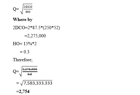
This means for each order placed, it should contain 2,754 units for product Y

Example 2

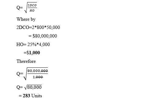
Milan Co ltd demand for raw material WW-12 is 50,000 litres per year. The cost per liter of this material is $4,000 and the holding cost per annum is 25%. If the ordering cost per order is 800. Compute the EOQ

Solution

Advantages of EOQ Model

1. Cost of production is reduced; EOQ model aids in scheduling of purchases which reduce inventory costs.
2. Reduction on chances of stockouts; when EOQ model is utilized, cases of shortages in supply is minimal and this avoids loss of sales.
3. Optimal utilization of resources. EOQ help in ensuring that resources such as cash is efficiently used. This avoids idle cash being tied in inventory.
4. Safeguarding the firm market share. Use of EOQ helps in ensuring that planning of future purchases for continuous supply is guaranteed. This ensures that no single period supply will decline. Hence, market share is stable or increase.
5. Opportunity cost. The EOQ model is a good investment tool for the firm can assess the opportunity cost associated with investing in inventory.

Disadvantages of EOQ Model

1. Complexity in computing. The model is a complicated one hence not commonly applicable in many businesses.
2. There are several assumptions made for this model which may not apply in the real-life situation.
3. It purports that it can forecast demand levels. The assumption that demand is constant may not be practical for it is influenced by many factors which have not been captured in this model.