Material Inventory Valuation Procedure-Simple Average Inventory Valuation Method

Specific objective; definition; simple average inventory valuation method; example

Specific Objectives

This article is guided by the following 2 specific objectives. The learner/user of this article will be able to;

1. Define the term simple average inventory valuation method
2. Compute inventory monetary value using simple average method

Simple Average Inventory Valuation Method

Definition

Simple average inventory valuation method is an approach which entails determination of a new average/mean price to be used for issuance in every inventory issuance transaction that takes place in the business.

FIFO Method is followed when selecting the price to include and the one to exclude in the computation. This means that if a batch of inventory is exhausted on issuance, its price is excluded in the computation of the new price to be used in the proceeding inventory issuance. On the same breath, if a new batch of inventory is received, its corresponding price is included in the computation of the new price if found applicable at that moment.

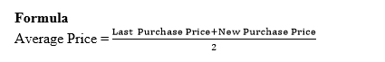
Formula for simple average price=Price of previous stock + Price of New Stock.

NB₁: The computed average price applies only when an issue is being made.

NB₂: Determination of Balance Brought Down (Inventory)=Previous inventory monetary Balance Less Monetary Value of Issued Inventory.

NB₃: A simplified way of determining the average issuance price is to consider the prices associated with the receipts of inventory and apply Pick and Drop methodology as you match the inventory balances.

Example

Polite Notice (PN) company ltd provided you with the following inventory details for the month of August 2021

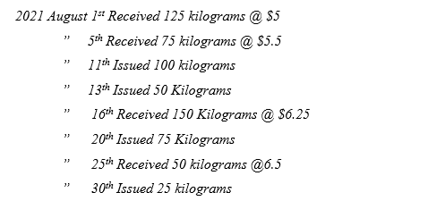
Required

Using the above information, determine the monetary value of closing inventory at the end of August under Simple Average method.      

Solution

The solution to this question requires you to compute the simple average price as shown below

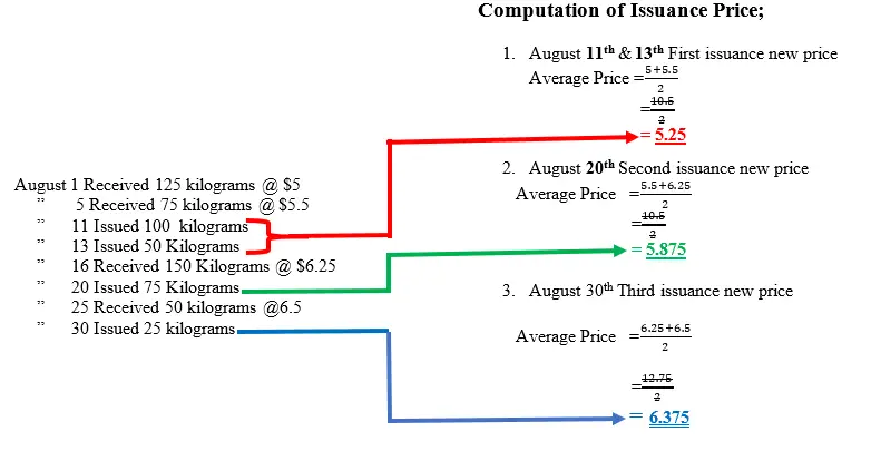
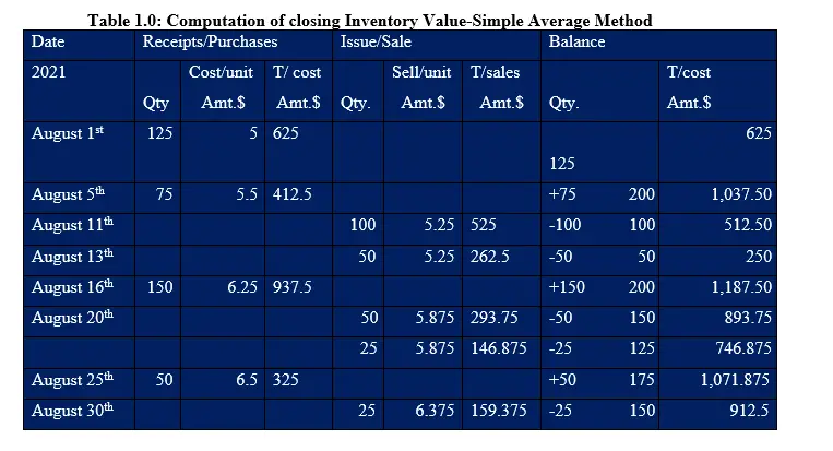
Explanation of Inventory Issuance-Simple Average Method above

Note: That, total units of inventory before issuance began was 200 units made up of 1^stAugust 125 units plus 5^th August 75 units. Then…

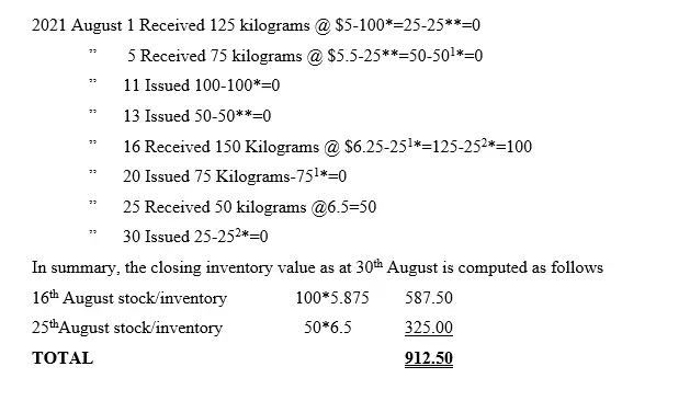
11^th August the first 100 units of inventory was issued and was from the 1^st August 125 batch of units of inventory received. The balance after that issuance was 25 units of inventory. On 13^th August the next issuance of 50 units of inventory was made and was from two batches; first, 25 units were gotten from the 1^stAugust batch of inventory whose balance was 25 units and second, the remaining 25 units was picked from the 5^th August batch. On 16^th August, received additional 150 units of inventory. So, the current total units of inventory are 50+150=200. On 20^th August, another issuance of 75 units of inventory was made. So, 50 units were picked from the 5^th August batch of inventory which had a balance of 50 units. This batch got exhausted. Therefore, the remaining 25 units to be issued was from the 16^th August inventory batch where by the balance was 125 units. Then another additional inventory was received on 25^th August of 50 units translating to a total of 175 units of inventory. Then the last issuance was an inventory of 25 units which was picked from the 16^th August batch which resulted to a final balance of 100 units. So, after the last issuance, we had a balance of 150 units in total (made up of 100 units of 16^th August batch plus 50 units of 25^thAugust batch).

Note that the superscripts (i.e., *, ** ,1* and 2*) used below will guide you on which inventory batch each issuance was picked from. This inventory analysis is a computational resilient of monetary value of closing inventory as at 30^th/08/2021.