Hypothesis testing decision rule (rejection or acceptance) of the null hypothesis-z score
1.1 Introduction
For you to comprehend on how-to carry-on hypothesis testing using z-score approach, you need to internalize some basic terms. Ask yourself, what is a Z-Score? What is Normal distribution? Assumptions and then How do you test the Null Hypothesis?
1.2 Basic terms used in Null Hypothesis testing-Z Score.
Some key and basic terms that are used in Null Hypothesis testing procedure are as described;
1.2.1 Z-Score
A Z-score is also referred to as Z statistic and it is an arithmetical gauge that designates a certain value's relationship to the average or mean of a group of values. A z-statistic, or z-score, is a number representing the result from the z-test. The Z-score relationship is in terms of dispersion of this aforesaid value away from the mean using standard deviations. For example, if a Z-score or statistic is 0, it implies that the data point's score is the same as the mean score. If the Z-Score is 1.96, then it means that the data point's score is 1.96 far away from the mean score.
NB: That a Z-Score is the proxy that is used when testing a Null Hypothesis.
1.2.2 Z-Test
Z test is a statistical examination or assessment used to determine whether two population averages or means are different based on two conditions, that is, one; the variances are known and two; the sample size is large.
1.2.3 Central Limit Theorem (CLT)
Central Limit Theorem (CLT) is a probability theory which advocates that as a sample increases, it approaches the normal distribution. i.e. the Bell curves.
1.2.4 Normal Distribution
Normal distribution is a probability distribution (i.e. Gaussian distribution), that portrays a certain expected manner of distribution of data from the population. It is a symmetric distribution around the mean, implying that the data around the mean has a higher frequency than the one on the extremes of the curve. Graphically, normal distribution has a bell shape and the standardized normal distribution has two parameters, namely; the mean and the standard deviation whereby for observations of around 68% of the total are represented by a +/- one standard deviation (1) away from the mean. A 95% are within +/- two standard deviations (2) away from the mean, and towards the tail ends, a 99.7% are within +/- three standard deviations (3). Normal distribution is anchored on the Central Limit Theorem.
1.2.5 Normal Curve
Normal curve is a graphical model that represents normal distribution of observations in the natural phenomenon. Normal curve portrays the characteristics of constructs containing continuous random variables. Most of the subject matters we study are dominated by behavior which follow a normal distribution and can be presented using a normal curve. A normal curve is Bell shaped as follows;
1.3 Assumptions of Z test
- For Z-test to work, the following assumptions are put in place;
- Data used is normally distributed
- Standard deviation which is a nuisance parameter is known
- Sample size is large or obeys the central limit theorem (CLT).
- Samples equal to or greater than 30 (x≥30) is sufficient enough to predict the characteristic/behavior of the population more accurately.
- Variables represented are identical and random.
Null hypothesis testing-z score
Decision rule of either accepting or rejecting the Null Hypothesis is twofold. Case one is where the data follows normal distribution and the number of observations or sample size is more than 30. Case two is where the data does not follow the normal distribution (t-distribution) and has a sample of less than 30. In this article, the focus is on case one where data is normally distributed. In this case, Z-Score is utilized in Null Hypothesis testing.
2.1 Acceptance or Rejection Decision Rule
Null Hypothesis testing end result is either Accepting or Rejecting the Null Hypothesis. That is;
If Sample Statistic Computed falls on the acceptance region, it means that Null Hypothesis is ACCEPTED
OR
If Sample Statistic Computed falls on the Rejection region, it means that Null Hypothesis is Rejected. So, how do we go about this?
Let’s Now Touch the Base!
Approaches of null hypothesis testing-z score
The question that arises is one, what criteria do we use to decide on whether to Accept or Reject a Null Hypothesis or the Alternative Hypothesis?
There are THREE approaches of hypothesis testing and each approach requires different subjective criteria and objective statistics although conclusion in all the three approaches is the same.
3.1 Test Statistic Approach
The classical test statistic approach computes a test statistic from empirical data and then compares it with a critical value.
Decision Rule: If the test statistic is larger than the critical value or if the test statistic falls into the rejection region, the Null hypothesis is Rejected.
3.2 P-Value Approach
In the p-value approach, researchers compute the p-Value on the basis of a test statistic and then compare it with the significance level (test size).
Decision Rule: If the P-Value is smaller than the significance level (P≤0.05) (usually α varies between 0.05 or 0.10 or 0.01), the researcher Reject the Null Hypothesis.
NB: A p-value is considered as the amount of risk that a researcher has to take when rejecting the null hypothesis.
3.3 Confidence Interval Approach
Confidence interval approach involves construction of the confidence interval and examining if a Hypothesized value falls into the interval region. The Null Hypothesis is Rejected if the hypothesized value does not exist within the confidence interval.
Generally, the Two-Tailed Test Null and Alternate Hypotheses are expressed as follows;
H0: Population parameter = Some Value
H1: Population parameter ≠ Some Value
3.4 Types of Null Hypothesis test-Z-Score
Null Hypothesis testing is performed based on the number of critical values used and the direction in which the critical value is located in the normal distribution curve. There are therefore three Null Hypothesis tests, namely;
Two Tailed Test
Right One-Tailed Test
Left One Tailed Test
3.5 Step by Step Procedure for Two Tailed Null Hypothesis Test
Generally, for two tailed test Null Hypothesis, the expression is as follows;
H0: Population parameter = Some Value
H1: Population parameter ≠ Some Value
For a case of two tailed test, the following steps will guide you on the decision rule to use.
STEP 1: Consider the Sample Statistics Available
The sample statistics can be either provided especially in an examination set up or it can be computed if one has done actual data collection for the sample.
STEP 2: State both the Null and the Alternate Hypotheses
This is the process of hypothesizing the study and both the Null and Alternate hypotheses are framed as follows;
H0: Population parameter = Some Value
H1: Population parameter ≠ Some Value
STEP 3: Determine the Level of Significance
Significant level always ranges between 0.10 up to 0.01
STEP 4: Compute the Critical Values (i.e. Theoretical-Z Values) for both sides; Right and Left-hand side of the normal curve
This objective can be achieved by using  and from the results gotten, confirm the corresponding z values (should be two for 2-Tailed Test i.e. non directional Z score with both plus and minus sign ±).
STEP 5: Compute the Critical Values (i.e. Computed-Z Values) for both Right- and Left-hand side of the normal curve
This value is computed for the purposes of comparing it with the theoretical value gotten in step 4 above so as to make the right decision.
The computation can be either manual using  formula or computerized. That is using computer software.
STEP 6: Make Decision Based on the Place Value of the Computed Z-value
In this step, compare the value of computed critical (i.e. Z computed score) value and the theoretical critical (i.e. Z Table Score) value.
STEP 7: Decision Rule;
If Z-Computed falls on the Rejection Region, i.e. Z-Computed value is greater than the Critical/ theoretical Value, Reject the Null Hypothesis. Otherwise ACCEPT.
Example 1 (A case of equal (=) or Two Tailed test)
Nocturnal Investors ltd is a group of keynote retired men who have been investing in diverse portfolio in the money market. Their portfolio manager feels that for the last ten years, returns have been performing equally to the peer average. He proclaims that on average, performance of the securities invested match the entire market (i.e. population). A sample of performance for 64 investment assets were obtained and the average returns was found to be $106 per annum, with standard deviation 20 and the level of significance was at 0.05.
Assuming that the population parameter (population mean-µ) performance was $100 per Annum.
Required
Test the Null Hypothesis
Solution
Can put it this way;
One;
H0: The average market performance is $100 per annum.
(Hint: When we say market performance, we mean the population mean).
OR
Two;
Null Hypothesis: There is no significant difference between the average performance of Nocturnal Investors Ltd portfolio and that of the market/population.
Empirically H0: μ= 100 OR
H0: μ=The average market performance is $100 per annum.
OR
Three;
Null Hypothesis: There is no significant difference between the average performance of Nocturnal Investors Ltd portfolio and that of the market (the population).

On the other hand, the alternative hypothesis can be expressed as;
One;
HA: The average market performance is NOT $100 per annum.
OR
Two;
Alternative Hypothesis: There is significant difference between the average performance of Nocturnal Investors ltd portfolio and that of the market.
Empirically HA: μ≠ 100
OR
Three;
HA: ≠µ
≠µ
Having gotten that concept of hypothesizing correctly, let’s move on to the next level of determining the Critical Value given the significance level.
At Level of Significance being α=0.05
Then Critical Value;
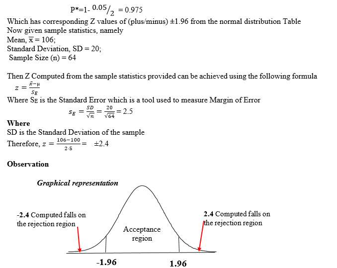
Decision Rule
The obtained Z-value Computed of 2.4 falls in the critical region (1.96), so the Null Hypothesis is rejected.
Conclusion
Hence, we conclude that there is significant difference. This means we adopt/accept the Alternate hypothesis.
3.6 Step by Step Procedure for Right Tailed Null Hypothesis Test
Generally, the Right One-Tailed Test Null and Alternate Hypothesis is expressed as follows;
H0: Population Parameter ≤ Some Value (Greater than or Equal to- Rule).
HA: Population Parameter > Some Value.
Step by Step Procedure for Right One Tailed Test-Null Hypothesis
For a case of Right One Tailed Test, the following steps will guide you on the decision rule to use.
STEP 1: Consider the Sample Statistics Available
The sample statistics can be either provided especially in an examination set up or it can be computed if one has collected data for the sample.
STEP 2: State both the Null and the Alternate Hypothesis
This is the process of hypothesizing the study and both the Null and Alternate hypotheses should be frames as follows;
H0: Population Parameter ≤ Some Value (Greater than or Equal to- Rule).
HA: Population Parameter > Some Value.
STEP 3: Determine the Level of Significance
This level exists as either 0.1; 0.05 or 0.01
STEP 4: Compute the Critical Values (i.e. theoretical-Z Values) for Right hand side of the normal curve
This objective can be achieved by using P*=1- α and from the results gotten, confirm the corresponding Z values (should be Right-One-Tailed Test).
STEP 5: Compute the Critical Values (i.e. Computed-Z Values) for both Right- and Left-hand side of the normal curve
This value is computed for the purposes of comparing with the theoretical value derived at in step 4 above so as to make the right decision. The computation can be either manual using  formula
or computerized, i.e. using computer software.
STEP 6: Make Decision Based on the place value of the Computed Z-value
In this step, compare the value of computed critical (i.e. Z computed score) value and the theoretical critical (i.e. Z Table Score) value.
STEP 7: Decision Rule;
If Z-Computed falls on the Rejection Region, i.e. Z-Computed value is greater than or equal to the Critical, theoretical Value, Reject the Null Hypothesis. Otherwise ACCEPT
You should know this; For Right One-tailed Test-always
HO: It is claimed/postulated that the sample statistic is greater than (≤) or equal to Population Statistic
Example 2 (A case of greater than or equal (≤) or one Right-Tailed test)
Let us assume the example of Nocturnal Investors ltd which is a group of keynote retired men who have been investing in diverse portfolio in the money market. Their portfolio manager feels that for the last ten years, returns have been Out-Performing above the peer average. He proclaims that on average, performance of the securities invested over match the entire market. A sample of performance for 64 investment assets were obtained and the average returns was found to be $106 per annum, with standard deviation 20 and the level of significance was at 0.05.
Assuming that the population parameter for performance was $100 per Annum.
Required
Test the Null Hypothesis
Solution
Can put it this way;
One;
H0: The average market performance is Greater than $100 per annum.
OR
Two;
Null Hypothesis: The average performance of Nocturnal Investors ltd portfolio is Greater than that of the market.
OR
Three;
Empirically H0: μ ≤ 100
On the other hand, alternative hypothesis states that;
One;
HA: The average market performance is Less than $100 per annum.
OR
Two;
Null Hypothesis: There is significant difference between the average performance of Nocturnal Investors ltd portfolio and that of the market.
Empirically H0: μ>100
At Level of Significance being α=0.05
Then Critical Value;
P*=1- 0.05 = 0.95
Which has corresponding Z values of (plus/minus) +1.64 from the normal distribution Table
Now given sample statistics, namely
Mean, ?x = 106;
Standard Deviation, SD = 20;
Sample Size (n) = 64
Then Z Computed from the sample statistics provided can is achieved using the following formula
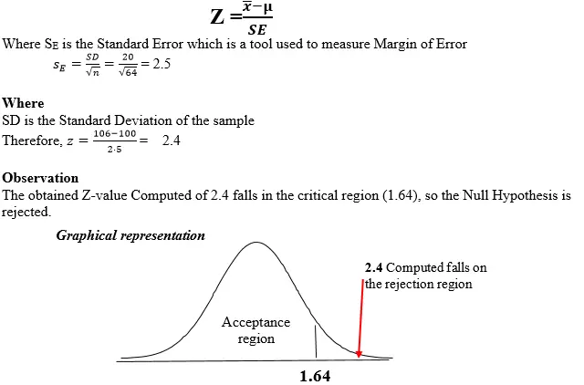
Decision Rule
Hence, we concluded that there is significant difference. In other words, the average performance of Nocturnal Investors Ltd portfolio is Greater than that of the market or in short, we say it is more than $100 per annum.
3.7 Step by Step Procedure for Left One Tailed Test-Null Hypothesis
Generally, the Left One-Tailed Test Null and Alternate Hypotheses are expressed as follows;
H0: Population Parameter ≥ Some Value (Less than or Equal to-Rule)
HA: Population Parameter < Some Value
For a case of Left One Tailed Test, the following steps will guide you on the decision rule to use.
STEP 1: Consider the Sample Statistics Available
The sample statistics can be either provided especially in an examination set up or it can be computed if one has collected the sample.
STEP 2: State both the Null and the Alternate Hypothesis
For the two hypotheses, they are expressed as;
H0: Population Parameter ≥ Some Value (Less than or Equal to-Rule).
HA: Population Parameter < Some Value
STEP 3: Determine the Level of Significance
This level exists as either 0.1; 0.05 or 0.01
STEP 4: Compute the Critical Values (i.e. theoretical-Z Values) for Left hand side of the normal curve
This objective can be achieved by using P*=1- α and from the results gotten, confirm the corresponding Z values (should be Left-One-Tailed Test).
STEP 5: Compute the Critical Values (i.e. Computed-Z Values) for both Left- and Left-hand side of the normal curve
This value is computed for the purposes of comparing with the theoretical value derived at in step 4 above so as to make the right decision. The computation can be either manual using formula
or computerized, i.e. using computer software.
STEP 6: Make Decision Based on the place value of the Computed Z-value
In this step, compare the value of computed critical (i.e. Z computed score) value and the theoretical critical (i.e. Z Table Score) value.
STEP 7: Decision Rule;
If Z-Computed falls on the Rejection Region, i.e. Z-Computed value is Less than or equal to the Critical, theoretical Value, Reject the Null Hypothesis. Otherwise ACCEPT
For Left One-Tailed Test-always
HO: It is claimed/postulated that the sample statistic is Less than (≥) or equal to Population Statistic
Example 3 (A case of Less than or equal (≥) or one Left-Tailed test)
Again, let us assume the example of Nocturnal Investors ltd which is a group of keynote retired men who have been investing in diverse portfolio in the money market. Their portfolio manager feels that for the last ten years, returns have been Under-Performing below the peer average. He proclaims that on average, performance of the securities invested under match the entire market. A sample of performance for 64 investment assets were obtained and the average returns was found to be $106 per annum, with standard deviation 20 and the level of significance was at 0.05.
Assuming that the population parameter for performance was $100 per Annum, test the Null Hypothesis.
Solution
Can put it this way;
One;
H0: The average market performance is Less than $100 per annum
OR
Two
Null Hypothesis: The average performance of Nocturnal Investors ltd portfolio is Less than that of the market
Empirically H0: μ ≥ 100
OR
Three;
HA: The average market performance is Less than $100 per annum
OR
Empirically HA: μ<100
At Level of Significance being α=0.05
Then Critical Value;
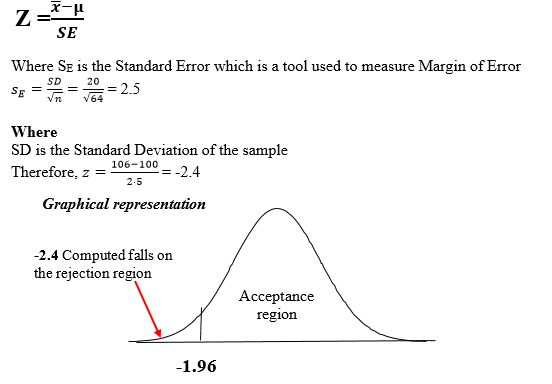
P*=1- 0.05 = 0.95
Which has corresponding Z values of (plus/minus) -1.64 from the normal distribution Table
Now given sample statistics, namely
Mean,= 106;
Standard Deviation, SD = 20;
Sample Size (n) = 64
Then Z Computed from the sample statistics provided can is achieved using the following formula
Decision Rule
The obtained Z-value Computed of -2.4 falls in the critical region (-1.64), so the Null Hypothesis is rejected.
Conclusion: Hence, it was concluded that there is significant difference. In other word the average performance of Nocturnal Investors Ltd portfolio is less than that of the market or in short, we say it is Less than $100 per annum.
Summary
In summary, this is the essence of Z-statistic test procedure. That the researcher want to establish statistically whether the claim he or she has is true or not by performing a hypothesis test. To achieve this objective, the researcher states both the null and alternative hypothesis, collect data from the whole population or from a sample if the population is too large to be managed.
So, what is the issue?
The issue is the claim being postulated.
That is, the change observed in the dependent or response variable/factor, is caused by the proposed independent/predictor variable.
Let me refer to our previous three examples of performance of Nocturnal Investors ltd which is a group of keynote retired men who have been investing in diverse portfolio in the money market.
In example one scenario: The claim is that there is equal performance between this individual investor (Nocturnal Investors Ltd) as compared to the overall/industry performance and that it should not be assumed that Nocturnal Investors ltd equal performance to that of the industry was due to chance but the portfolio manager had put significant efforts.
In other words, we are saying;
μ= 100 (the average performance of the industry/market is 100).
=100 (the average performance of the Nocturnal Investors Ltd is also 100).
And this is not by chance but it is by the statistically the significant role the Nocturnal Investors ltd portfolio manager has impacted in this single firm.
In example two scenario, it is a case of outperformance. We are saying Nocturnal Investors ltd is performing over and above the industry average and this performance which is above is not by chance but the portfolio managers of Nocturnal Investors ltd has impacted significant efforts or strategies to make sure the firm outperforms.
That is;
(the average performance of the Nocturnal Investors ltd is more than market/population average performance which claimed to be 100)
In example three scenario, it is a case of under-performance. We are saying Nocturnal Investors ltd is under performing below and the industry average performance and this performance which is below is not by chance but the portfolio managers of Nocturnal Investors ltd has NOT impacted significant efforts or strategies to make sure the firm performs.
That is;
(the average performance of the Nocturnal Investors Ltd is LESS than market/population average performance which claimed to be 100)