Hypothesis testing decision rule (rejection or acceptance) of the null hypothesis-t-test approach
1.1 Introduction
Let’s Now Touch the Base!
What is a t-test? Its applicability? Examples!
Definition
T-Test is a hypothesis testing tool for evaluating whether the mean of groups of observations have the same mean (measure whether there exists statistically significant difference) especially when the standard deviation of the population is unknown.
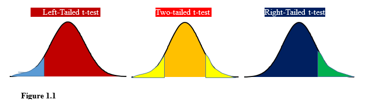
The t-test statistics can assume either a two tailed test or one-tailed test, either; Right or Left options as summarized in Figure 1.1 below
1.2 Applicability of t-test Hypothesis
Where does t-test apply? T-test applies where the sample size is equal or less than 30 units of observation.
t-test is inferential in nature and it incorporates the t-statistic, the t-distribution values, and the degrees of freedom to determine the statistical significance. If the means/averages are more than two, then the hypothesis tool that the researcher will use is ANOVA to conduct the test.
1.2.1 How t-test Works
The t-test helps you to evaluate whether two sets from the same population have mean with statistically significant difference. So, if for instance you consider two samples, namely group one and group two of students from the same class of Sociology. Then if we establish the means of the selected parameter for each group, we will not expect much deviation as far as the mean/average is concerned.
Before the determination of the two means is carried out, a t-test hypothesis will be developed, whereby the null hypothesis will state;
H0: There is no statistically significant difference between the mean of the two groups
i.e. this implies that the mean from the two sets of data are the same.
The alternate hypothesis will state as follows;
HA: The means from the two groups are statistically different.
With applicable formulas, you compute the relevant statistics and compare the same with the standard/theoretical values for your decision rule.
Decision rule is the last step to be considered in the whole process of hypothesis. In this case, the assumed null hypothesis will either be accepted or rejected.
Note: If the null hypothesis is accepted, it will imply that the difference between the two means from the population is not statistically significant, so the difference is due to chance only.
If the null hypothesis is rejected, it implies that the difference between the two means from the same population is statistically significant and that data readings are strong and are probably not due to chance. In this case, we go for alternate hypothesis which obviously states that the mean from the two groups from the same population is statistically different.
1.2.2 Key Data Values Required to Compute the t-Statistic
Mean Difference.
Standard Deviation of Each Group.
Number of Data Values of Each Group.
Outcome.
Computed/calculated t-value.
Critical value table t value (gotten from the t-distribution table).
1.2.3 Assumptions of t-test
The Data collected observes continuous or ordinal scale of measurement.
Samples selected from the same population is randomly selected.
Data is normally distributed. i.e. obeys the normal curve patterns.
Variance homogeneity of the two groups especially when the standard deviations of the two groups are the same.
Types of sample tests (under t-test)
Basically, there are TWO types of sample t-tests, namely;
1.One Sample t-test
2.Two Sample t-test:
One sample t-test
In the case of one sample t-test, we compare the mean or average of one sample with the mean or average of the population where the sample was picked and /or theoretical mean as stated in the null hypothesis.
2.1. Steps of One Sample-t-test
The following 8 step by step procedures will guide you to the correct decision.
STEP 1: Select the group of concern-this is the unit of observation, an individual or an individual representing an artificial person such as an organization.
STEP 2: Identify the characteristic you wish to observe/measure.
STEP 3: State both the Null Hypothesis (H0) and Alternate hypothesis (H1).
STEP 4: Collect data of the characteristic you are observing.
STEP 5: Compute the sample mean/average.
STEP 6: Actual Hypothesis testing process-Compare the sample mean with the population mean/average or if not given, use the theoretical average/mean value as stated in the Null hypothesis.
NOTE: To compare the two means, there are two approaches you can use, namely;
-Manual approach where the relevant values are computed using free hand.
-Computerized approach using computer programs such as Excel or SPSS
OPTION ONE
If use Manual Approach
Compute the t value using the appropriate formula (commonly referred to as Computed t-value)
Formula is
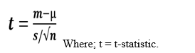
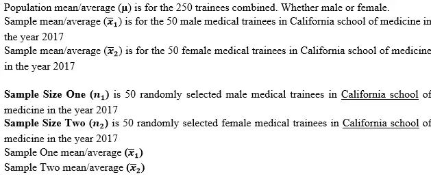
m = Group mean/average you have computed.
µ = Population mean/average given or use theoretical mean as stated by the null hypothesis.
s = Group standard deviation.
n = Sample size of the group used.
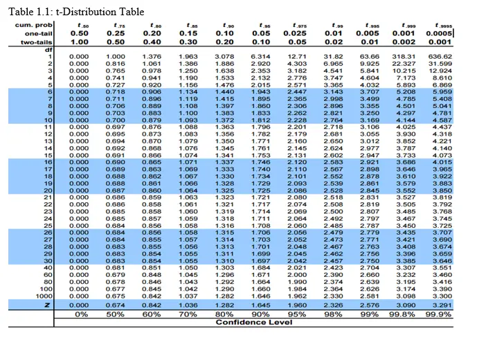
STEP 7: Identify the corresponding Critical Value (commonly referred to as theoretical t-value) from the t-test Table (remember degrees of freedom-df=N-1 against level of significance as provided).
Remember it is capital N not small n for our case is of One Sample t-test which is compared with the population (N) mean.
See Table 1.1: t-Distribution table below.
STEP 8: Decision Rule
Alternative one: If the computed critical value is greater than the theoretical critical value (the one read from the t-table), then
Reject the (i.e. Fail to Accept) Null Hypothesis. This implies that there is statistically significant difference between the sample mean and the population or theoretical mean and so the grand meaning is that the difference between the two means/averages is caused by other factors other than chance alone.
Alternative two: If the computed critical value is LESS than the theoretical critical value (the one read from the t-table, usually 5% or 0.05), then
ACCEPT the (i.e. Fail to Reject) Null Hypothesis. This implies that there is no statistically significant difference between the sample mean and the population or theoretical mean and so the grand meaning is that the difference between the two means/averages is caused by chance alone
OPTION TWO
If use Computerized Approach-Using SPSS
Go to Analyze option -> Compare Means -> One-Sample T Test.
Drag and drop the variable you want to test against the population mean into the Test Variable(s) box.
Specify your population mean in the Test Value box.
Click OK.
Your result will appear in the SPSS output viewer.
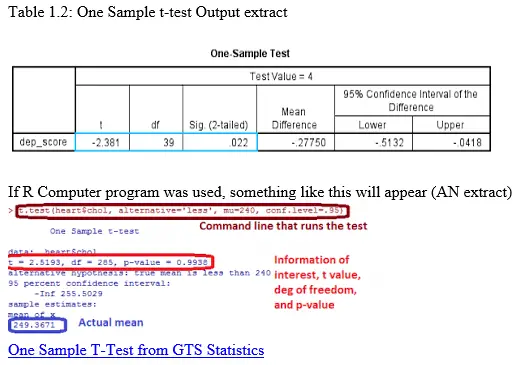
NB1: Final output appears as something like this if SPSS computer program was used
NB2: Always ignore the t sign (whether + or -) gotten from the computer program output. See Table 1.2 below
CONCLUSION
The computerized results are the same as the manual approach one.
NB: Using p-value approach from the computer-generated output,
If the computed critical value is greater than the theoretical critical value (the one read from the t-table), leading to rejection of the null hypothesis, then
Corresponding p-value will be smaller than the critical value (where by most of the times it is 0.05), hence we still reject the null hypothesis as it is in the case of manual approach. The vice versa is true.
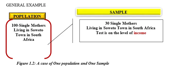
From the above pictorial demonstration, as shown by Figure 1.2, there may be a claim by the government that single mothers living in SOWETO town have low income and need government intervention. This is a government decision to be implemented, but the concerned government officials are not sure how true this claim is. So, if you are invited as a research consultant to empirically proof to what extent that claim is true or false, you need to set and achieve the following objective;
Objective; To test whether the sample mean/average (i.e.) income of the 30 women randomly selected is equal to the population mean/average (i.e. µ) of the 100 women taken as the population
Why test?
You see the problem here is that we do not want to pick a sample and on carrying a t-test on it, the results portray low income status which may be due to chance. While in fact, we may even have the majority of the single women having high levels of income apart from a few who are struggling with low income. So we want as we do the test, to be sure that the results we get can be generalized for the population. Therefore, justification of testing is to be sure that the mean/average income as claimed by the government for the whole population is true by just carrying a t-test procedure using a sample.
Before we go very far with our discussion, allow me I do some clarification.
.
When we talk of mean/or average, what is this? Mean, refers to Expected outcome. When we compute mean of a certain value, let’s say X, we are talking of the expected outcome of variable “X”. For example, when we say mean/average income of employees, we refer to the expected income of employees. Is that understood?
Let me take you an extra mile. Further, when we say expected income, the term expected further refers to normal income. Normal from the word “normal distribution” or “normal curve”. You know about normal curve.
So, when we are determining mean/average value, we are determining what is normal and what is normal is what is expected.
Back to our track….
In our SOWETO case, the researcher needs to test whether the 100 single mothers living in this town have low income of let say 1000 Rand per annum. This is what the government is claiming is the expected income of the population.
On the other hand, the researcher wants to proof or disapprove that by carrying a ONE SAMPLE t-test whether the mean/average/expected income of the 30 single mothers randomly selected (sample) have equal or the same mean or average or expected income of the 100 women in Soweto.
Therefore, the Null Hypothesis will state that the sample mean is the same as the population mean.
In other words,
If there is any difference in the means/averages, it will be due to chance only. In this case, we will accept the null hypothesis;
OR
If the null hypothesis is rejected, then it means that any difference in the means/averages, will not be due to chance only but other significantly contributing factors. In this case, we will reject the null hypothesis and adopt the alternative hypothesis.
Interpretation of the Results
So, you may ask, in both hypotheses, which one will the government decide to intervene or withdraw the intervention?
The Answer is as follows;
If the Null hypothesis is accepted, it means that even if the sample mean/average computed is different from the population mean/average, we ignore that difference for it is due to chance only and the researcher should advise the government to move on with the intervention decision.
Further Explanation…
This is what we are saying that since the difference gotten between the two means/averages is due to chance, we should conclude that the sample mean is the same as the population mean. In other word, the mean income gotten from the sample is the same as for the 100 women and so the government is well guided that all the single mothers in Soweto are actually poor and assistance is needed.
If the Null hypothesis is rejected, it means that the difference between the sample mean/average computed and that of the population mean/average, has not been caused by chance only but there are other strongly explaining factors. Hence this difference is statistically significant and the researcher should advise the government to stop intervening for truly we may have both rich and poor single mothers living in SOWETO.
Further Explanation…
This is what we are saying that since the difference gotten between the two means/averages is NOT due to chance alone, we should conclude that the sample mean is NOT the same as the population mean. In other word, the mean income gotten from the sample is NOT the same as for the 100 women and so the government is well guided that all the single mothers in Soweto are NOT actually ALL poor and therefore no assistance is needed for all the 100. This may call for a further investigation to discriminatively select only the ones who are actually poor and assist them.
Specific Example
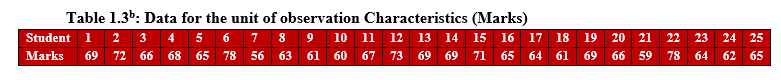
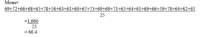
In a certain beauty contest, the principal of one of the commercial colleges who had students compete decided to find out if her students over performed due to chance or they were adequately prepared for the competition by going through rigorous practice. She selected a simple random sample of 25 students who scored an average of 66.4 on a homogenous test. The corresponding standard deviation was of 2.5. If the overall average for all the participants was 60.2.
The individual performance data for the students were as follows

Required
Determine whether this over performance was by chance or due to the rigorous practice.
Hint use both manual and computerized approaches
SOLUTION
STEP 1: Select the group of concern-this is the unit of observation, an individual or an individual representing an artificial person such as an organization.
Answer: Beauty contest group of students of a particular college
STEP 2: Identify the characteristic you wish to observe/measure
Answer: Performance in the beauty contest
STEP 3: State both the Null and Alternate hypotheses
Answer: H0: There is no statistically significant difference between the sample mean of the students who participated in the beauty contest and the population mean (i.e. mean of all the competitors
involved).
That is symbolically  -μ=0
-μ=0
OR
Answer: H0: There is no statistically significant difference between the sample mean of the students who participated in the beauty contest and the population mean (i.e. mean of all the competitors involved).
That is symbolically =μ
Answer: STEP 4: Collect data of the characteristic you are observing. See Table 1.3
Answer: STEP 5: Compute the sample mean/average
Answer: STEP 6: Actual Hypothesis testing process-Compare the sample mean with the population mean/average or if not given, use the theoretical average/mean value as stated in the Null hypothesis.
NOTE: To compare the two means, there are two approaches you can use, namely;
-Manual approach and
-Computerized approach using computer programs such as Excel or SPSS
OPTION ONE
If use Manual Approach
Compute the t value using the appropriate formula (commonly referred to as Computed t-value)
Formula is
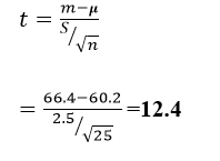
From t table, with DF=N-1=24 and significant level of 0.05 translates to
Critical 2.064
Decision rule
Since computed CV is greater than theoretical CV, we reject (i.e. fail to accept) the Null hypothesis which implies there is statistically significant difference between the sample mean and the population mean. In other words, the over performance was not due to chance alone, but also the rigorous practice that the students were exposed to.
OPTION TWO
Computerized Approach
Suppose we use the SPSS One sample t-test? Will the results be the same?
SPSS Output was as per Table 1.4
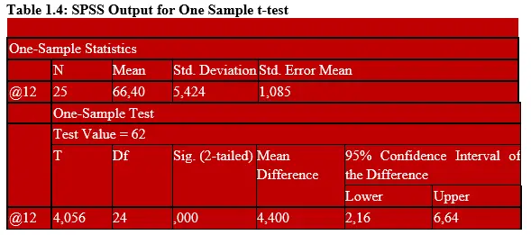
P value=0.000 which is smaller than the theoretical critical value of 0.05
Hence Reject the H0. So, you can see that the results translate to the same decision rule!
Two sample t-test
Unlike in the case of one sample t-test where only one sample is picked from one population set, a two-sample t-test is a statistical test used to compare the means/average of two populations by randomly selecting corresponding two samples for the t-test procedure to take place. The two-sample t-test is practical under some assumptions.
3.1 Assumptions of an Unpaired Two Sample t-test
- The data is continuous in nature
The researcher should rely on data of a continuous nature or scale. For example, when gauging mass, it is expressed in kilograms which can be expressed as 2kgs, 10kgs, 10.45kgs 23.33kgs. This is what is said to be continuous data.
- Comparison of Only two groups or samples
Unpaired t-test is only applicable where two groups are used. For instance, comparing a group of white and black individuals or married and unmarried people.
- Independence between the two groups or samples
There must be a demarcating line between the two variables based on some conditions or circumstances such as sex or medical treatment. For example, data can be collected for the group with treatment experience and those who have not received the treatment.
- Data collected should portray normal distribution
The two data set should demonstrate that they were collected from a normally distributed population.
- Equal variance between the two samples/groups should prevail
The standard deviation for the two samples or groups should be the same. That is, the variance between groups is the same.
3.2 Classification of Two Sample t-test
The two-sample t-test is further sub-divided in to (UP) categories. That is….
Unpaired sample t-test and Paired sample t-test. These are;
i). Independent two sample t-test
ii). Dependent two sample t-test
3.2.1 Independent Two Sample t-test (Unpaired t-test)
Independent two sample t-test also known as Unpaired t-test is a statistical test used to compare the means/average of two populations by randomly selecting corresponding two samples for the t-test procedure to take place. The variance of data is the same between the groups, meaning that they have the same standard deviation.
NOTE the following;
When we say the two samples are independent or different, it means that although the two samples may be randomly selected from either the same physical population set or from two different physical population but sharing the same characteristics with the other one (we will see this scenario shortly) it means the two samples are simply treated or subjected to different condition before the mean of the characteristic of the researcher’s interest is tested.
In other word we are saying that;
The two samples are drawn from the same population (i.e. of course assumed to share similar characteristic), but subjected to different treatment.
OR
The two samples are drawn from the different population, (i.e. of course assumed to share similar characteristic), but subjected to the same treatment.
Examples
Independent such as SEX e.g. Male and FEMALE respondents-common characteristic being blood sugar levels between the two groups.
Independent such as White athletes and Black African athletes-common characteristic being frequency of winning a race.
Independent such as trained and untrained teachers-common characteristics being the levels of income per annum.
Methodology of Data Collection
Method or approach used to collect data in the case of Independent Two Sample (t-test (Unpaired t-test) may differ from one researcher to another. Let’s look at the following scenarios
Scenario 1: Both Sample One and Sample Two from One Population
This is demonstrated by Figure 1.3 as follows;
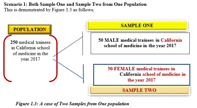
In Figure 1.3, from one population, “TWO” independent samples in terms of SEX are randomly selected from the same type of population for t-test.
IQ Level of medical trainees is the Characteristic being observed which is represented by
X1 is the level of IQ of trainees from California
X2 is the level of IQ of trainees from California
Population size (N) is 250 medical trainees in California school of medicine in the year 2017
NB: That the two samples were both picked strictly from one population set (Universe). As the name suggests, the t-test is referred to as independent two sample t-test because the condition or aspect of sex is so distinct such that in normal circumstances, we only have two categories of mankind, male or female. This is a case of unpaired two samples t-test.
Scenario 2: Both Sample One and Sample Two from Two Populations
This is demonstrated by Figure 1.4 as follows;
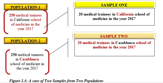
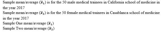
In this case of Figure 1.4, from two populations (California and Casablanca), Two independent samples in terms of SEX are randomly selected for the t-test.
IQ Level of medical trainees is the Characteristic being observed which is represented by
X1 is the level of IQ of trainees from California
X2 is the level of IQ of trainees from Casablanca
Population size (N1) is 250 male medical trainees in California school of medicine in the year 2017
Population size (N2) is 250 female medical trainees in Casablanca school of medicine in the year 2017
Population mean/average (µ1) is for the 250 California medical trainees combined. Whether male or female.
Population mean/average (µ2) is for the 250 Casablanca medical trainees combined. Whether male or female.
Steps for Independent Two Samples T-Test (A Between Case)
The following 9 step by step procedures will guide you to the correct decision.
STEP 1: Select the group of concern-this is the unit of observation, an individual or an individual representing an artificial person such as an organization.
STEP 2: Identify the characteristic you wish to observe/measure
STEP 3: State both the Null and Alternate hypotheses
STEP 4: Collect data of the characteristic you are observing
STEP 5: Compute the sample mean/average for both samples
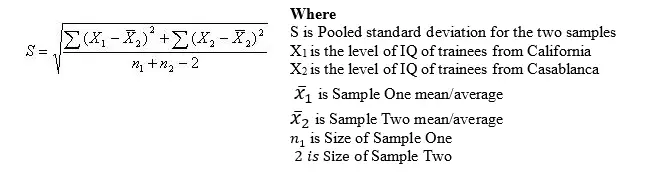
STEP 6: Compute standard deviation (S) for both independent groups or samples. Appropriate formula is;
NOTE: To compare the two means, there are two approaches you can use, namely;
-Manual approach
-Computerized approach using computer programs such as Excel or SPSS.
OPTION ONE
If use Manual Approach
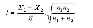
STEP 7: Compute t-statistic value
STEP 8: Determine Degrees of Freedom (DF)
V= (n1 + n2)-2
Where;
V= is the degree of freedom whereby the sample set a are two
n1= Sample size of sample one or group one
n2= Sample size of sample one or group one
At certain confidence level-most of the time 95% (i.e. 0.05)
STEP 9: Actual Hypothesis testing process
With the calculated t-test value, compare it with the theoretical t-test value (i.e. 0.,05 for instance).
OPTION TWO
If the computed t-test value is LESS than theoretical (also referred to as table value, ACCEPT the Null hypothesis. Otherwise REJECT.
If computerized Approach is used e.g. SPSS program
Click on the “SPSS window and follow instructions thereof
Example 1
Peter James is a nutritionist working in a public hospital in Canada. He carried out a research to find out the level of fat for hospital inpatients. To achieve this objective, he considered two groups of in-patient consumers of fatty foods and those who are vegetarians. He therefore selected 10 people from each category (from two populations-i.e. fatty food and vegetable food eaters in that order). The amounts of fat content per month was recorded as follows;
Fatty food eaters (F): 105, 220, 135, 110, 220, 92,80,158, 75, 150
Vegetarian eaters (V): 108, 245, 125,142, 144, 175, 200, 175, 101, 130
The average/mean for the fatty food eaters was 135 with a standard deviation of 52.91. The mean for the vegetarian food eaters is 155 with a standard deviation of 44.55.
Required
Test the null hypothesis
Solution
Remember that this is a case of unpaired t-test (i.e. independent two t-test) because the two eating habits are independent/different from one another. Also remember that the common characteristic in the two samples is the fat level in the body.
H0: The mean/average fat level between Fatty food eaters and Vegetarian eaters is not statistically significant.
HA: The mean/average fat level between Fatty food eaters and Vegetarian eaters is statistically significant.
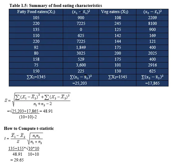
From the t-distribution Table at 5% and DF=20-2=18
t=2.101
Decision Rule
Reject the Null hypothesis.
3.2.2 Dependent two Sample t-test (Paired t-test)
Dependent samples t-test is often referred to as "Paired t-test". This is a two-sample t-test whereby the two samples are selected from the same population. In other words, for paired t-test point of view implies that both samples consist of the same test subjects. Therefore, the data generated is such that for each data point in one sample is outstandingly paired to a data point in the second sample. Further, as the term suggests, the variable used in the measurement are referred to as dependent variable, (continuous) for there is a dependency element thereof.
Assumptions of Dependent two Sample t-test (Paired t-test)
Paired Two Sample t-test is anchored on several assumptions which makes the concept practical. They include and not limited to;
i). Dependent variable also known as criterion variable should be of continuous (interval or ratio) in nature.
ii). Dependent variable also known as criterion variable should obey normal distribution.
iii). Dependent variable also known as criterion variable should not have cases of outliers.
iv). Observations collected should be independent of each other.
Classification of Dependent Two Sample t-test (Paired t-test)
Dependent Two Sample t-test (Paired t-test) is further divided in to two more sub-categories, namely;
Paired “Difference” t-test
Repeated “Measures" t-test
(a). Paired “Difference” t-test
In this type of paired t-test, the two samples, sample one and sample two are randomly selected from the same population whereby one sample is set aside and classified as the control sample. While the other sample is subjected to the required condition. Then their mean/average for the common characteristics is tested. This t-test is also referred to as correlated t-test because the two samples have similarities for testing purposes.
Methodology of Data Collection
Method or approach used to split the population into two samples differ from one researcher to another. Let’s look at the following scenarios
Scenario 1: Sample One and Sample Two from One Population
This is demonstrated by Figure 1.5 as follows;
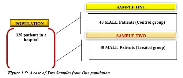
In Figure 1.5, sample one is picked from the population and sample two is picked from the same population. For instance, if the researcher wants to test for blood sugar level of in-patients in a certain hospital, he can select a group of 40 male patients and another group of 40 male patients from the same hospital. One group/sample is taken to be the (control group) and the other group is treated (treated group) with blood sugar control medical treatment and then the two groups are compared.
Scenario 2: Sample One from Population Split into Sub-Sample One and Two
This is demonstrated by Figure 1.6 as follows;
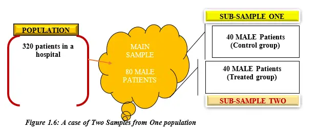
In Figure 1.6, the main sample is picked from the population and then it is split into two sub-samples as shown up here. For instance, if the researcher wants to test for blood sugar level of inpatients in a certain hospital, he can select a group of 80 male patients and further split in to two more sub-samples. One group/sample is taken to be the control group and the other is treated with blood sugar control medical tablets and then the two groups are compared.
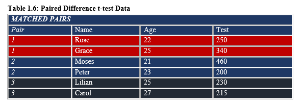
Illustration 1
This illustration 1 portrays the case of Paired Difference t-test as per Table 1.6
(b). Repeated “Measures" t-test
It is also called “Repeated Measures" t-test. The repeated measures t-tests are applicable where the same item or group is tested twice, hence the test is commonly referred to as a repeated measures t-test. For instance, testing the effectiveness of medical treatment of one subject or group of individuals before and after the pharmaceutical treatment. In this case, the same group of people are used.
NOTE the following;
When we talk of two samples which are dependent or the same, what does this imply?
Two samples; mean the same sample selected from one type of population is used to collect two sets of data where by the subject matter is tested twice. So, the two sets of data represent two samples. This is not like case of unpaired t-test where the two samples can either be from the same population or from two similar populations.
Dependent; means the researcher will use the same sample randomly selected from the population to collect and test the first and second data sets needed.
Example
A subject matter is tested prior to a treatment, say vaccinated against Covid-19 attack, and the same subjects are tested again after vaccination to find out whether with a Covid-19 injection will really-lower chances of conducting the pandemic. By comparing the same patient's numbers before and after treatment, we are efficiently using each patient as their own control.
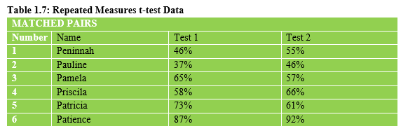
Illustration 2
This illustration 2 portrays the case of Repeated Measures t-test as per Table 1.7
3.3 Importance of Paired Samples t-test
These types of t-test are useful in manifold ways, namely;
i). The researcher will make us of this tool to measure the statistical difference between two time points in time.
The researcher will make us of this tool to measure the statistical difference between two conditions.
The researcher will make us of this tool to measure the statistical difference between two measurements.
The researcher will make us of this tool to measure the statistical difference between a matched pair
3.3.1 Hypothesizing a Paired Sample t test
Framing of the hypothesis can take two forms
For Null Hypothesis, we will have, H0: µ1 = µ2 (The paired population means/averages are equal") while the alternative hypothesis will read as follows;
Alternate hypothesis, H1: µ1 ≠ µ2 (The paired population means/averages are not equal")
OR
The two hypotheses can be re-written as follows;
For the null hypothesis; H0: µ1 - µ2 = 0 (The difference between the paired population means is equal to 0)
For the Alternate hypothesis; µ1 - µ2 ≠ 0 (The difference between the paired population means is not 0)
Where
µ1 is the population mean of variable 1, and
µ2 is the population mean of variable 2.
Steps for Dependent two Sample t-test (Paired t-test)
The following 8 step by step procedures will guide you to the correct decision.
STEP 1: Hypothesize the Paired Sample t-test
STEP 2: Collect Data Required
STEP 3: For each pair, compute the difference of the observations thereof. i.e. (di = X1 -X2),
NB: Ensure you note both the negative and positive deviations.
STEP4: Determine the average/mean of the difference gotten in step 3 above
STEP 5: Compute the standard deviation by subtracting the mean gotten from differences values already determined in step 3. Caution, you do it like the way we compute normal standard deviation when we have the normal observations (s.d).
STEP 6: From step 5, determine the standard error of the mean difference
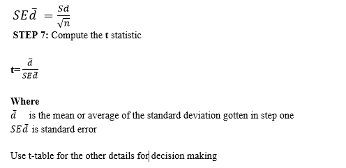
STEP 8: Decision Rule to accept or reject the null hypothesis
Example
A class of 20 Mechanical Engineering students were tested on their technical skills by carrying out a practical assignment in the lab before and after Computer Aided Technique was introduced. The short practical examination results were as presented in the Table 1.8a below
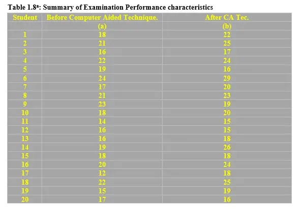
Required
Determine the t-computed value and compare with theoretical t-value and decide on the null hypothesis.
Solution
Hint: Manual Approach and it is a case of 2Tailed Test
Hypothesizing
For the sake of in depth understanding, let me present the framing of the hypothesis using the two approaches as discussed earlier in this tutorial
For Null Hypothesis, we will have, H0: µ1 = µ2 (The paired population means/averages are equal") while the alternative hypothesis will read as follows;
Alternate hypothesis, H1: µ1 ≠ µ2 (The paired population means/averages are not equal")
OR
The two hypotheses can be re-written as follows;
For the null hypothesis; H0: µ1 - µ2 = 0 (The difference between the paired population means is equal to 0)
For the alternate hypothesis; µ1 - µ2 ≠ 0 (The difference between the paired population means is not 0)
Where
µ1 is the population mean of variable 1, and
µ2 is the population mean of variable 2.
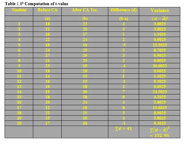
Computation of t value
OPTION ONE
Use of Manual Approach
From Table 1.8b below, the t-value is computed as shown herein
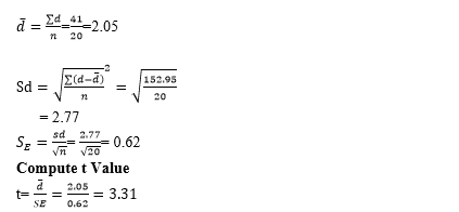
From the t-statistic distribution Table at 95% confidence level and df=20-1=19
Then the corresponding theoretical t value is;
t= 2.093
Decision rule-since the computed t-value is greater than the theoretical value. We reject the Null Hypothesis and conclude that there was strong evidence that, on average, the CAT introduced lead to great improvement which cannot be associated to chance alone.
OPTION TWO
Use of Computerized Approach-SPSS
Steps to be followed are as indicated below
STEP 1: Input data used in using the data view menu
STEP 2: Input variables used in using the variable view menu
STEP 3: Select Analyze Option then go to Compare Means button then click the Paired-Samples T-Test option window
STEP 4: Select the variable to be tested and click to transfer it to the right window as directed
STEP5: Choose the options to pick the appropriate confidence interval level, then click continue button
STEP 6: Go to “Click Ok” option and press once
The results will be as follows in this Table 1.7 below;
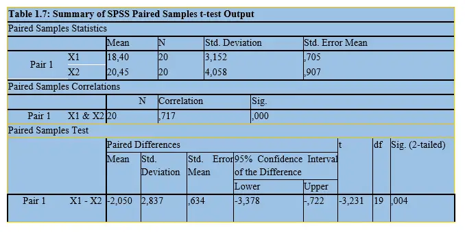
You can see that using the computerized approach, our p value is 0.004 which implies that the results are statistically significant for the value is less than the critical value of 0.05. Therefore, we rule that the null hypothesis to be REJECTED as it was in the previous case of manual approach.
Now, from this computer output, let’s make the following conclusion points which are very important
The mean of pair X1 is 18.40
The mean of pair X2 is 20.45
Correlation value of marks before and after introduction of computer aided technology is 0.717 which is a very strong positive relationship.
The difference in the mean/average between the marks gotten by the students before and after the CAT was -2,050 hence, we can conclude that the mean/average marks gotten by the students before the CAT was lower than the mean/average mark after introduction of CAT.
CONCLUSION
This t-test of Paired samples represents a test of hypothesis to establish whether the mean/average value of the same sample group has statistically significant difference or not. To achieve the aforementioned objective, the following criteria are of paramount importance;
The group members for the sample should be randomly selected
The data utilized has to be of interval and ratio scale
The 2 samples used should be from the same population
Data is normally distributed
Outliers cases are absent. In other words, no extreme values in the observations made.
Confirmation test for equality of variances
In two sample t-test, it is assumed that the variance or standard deviation between the two populations are equal. However, it is always advisable to confirm whether the variance between paired samples is equal or not equal before making use of the output thereof. To achieve this objective, test for Equality of Variances is utilized.
The hypotheses of these test are: -
Ho: σ1= σ2 (The standard deviations in the two populations are equal)
HA: σ1≠ σ2 (The standard deviations in the two populations are not equal)
On testing for equality, if the corresponding p-value is greater than the critical value (p>0.05), then it means that there is no adequate proof that the standard deviations in the two populations are different. In this case we will assume equal variances since we have no clear evidence to the contrary. In other words, we ACCEPT the null hypothesis that standard deviations in the two populations are equal. In this case, when we are conducting two-sample t-test to compare the population means, we use the test statistic for equal variances (Pooled t-test).
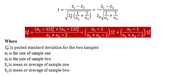
Equal Variance (Or Pooled) t-test
According to the hypothesis ruling above, that is if p-value is greater than the critical value (p>0.05), then it means that we ACCEPT the null hypothesis that standard deviations in the two populations are equal. As a result, pooled t-test is used when the number of samples in each group has the same variance, or the variance of the two data sets is similar then this formula is the most suitable for carrying out t-test.
The t-test statistic for a case of EQUAL VARIANCE is given by
Unequal Variance t-test
On the other hand, if the corresponding p-value is less than the critical value (p<0.05), then it means that there is adequate proof that the standard deviations in the two populations are different. In this case we will assume unequal variances since we have no clear evidence to the contrary. In other words, we REJECT the null hypothesis that standard deviations in the two populations are equal. In this case, when we are conducting two-sample t-test to compare the population means, we use the test statistic for unequal variances (Welch’s t-test).
Welch’s t-test
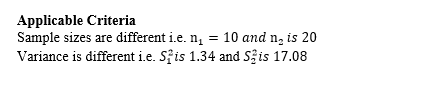
Welch’s t-test is applicable where the variances are not equal. It is used where
One; the sample size in each group under consideration is different. For example, sample one has 10 items and sample two has 13 items.
Two; the variance in each sample is also different from the other group. The following formula is used for calculating t-value and degrees of freedom for an UNEQUAL VARIANCE t-test:
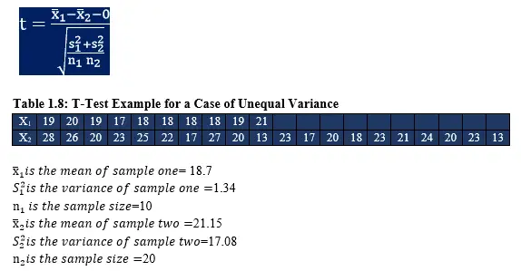
You can see that the average/mean of sample two (X2) exceeds that of sample one (X1). But this does not imply again that the corresponding mean of population two is higher than that of population one in that order.
May be the question that the researcher will be asking him/herself is whether the difference in mean from 18.7 up to 21.15 is due to chance alone, or do differences really exist in the overall populations.
Since the criteria portrays that the researcher is sure that the variances are dissimilar, then it means that it is NOT safe to assume that the two populations have equal standard deviations, then he/she will use Welch’s t-test as follows;
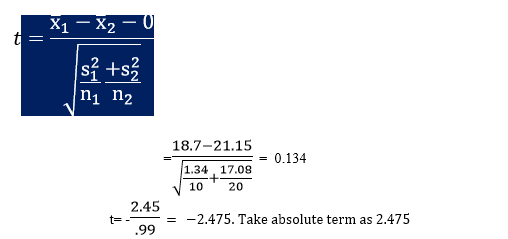
From the t-distribution Table, we read (10+20)-2=18, at 0.05, for Two tailed test=2.101
Since the computed t value is greater that the hypothetical or the t-table one, at a significance level of 5%. Therefore, it is safe to reject the null hypothesis that there is no difference between means. The population set has intrinsic differences, and they are not by chance alone.